Cycle Analysis
Background
Digital Signal Processing, or DSP as it is more commonly known, has been around since the the late 1940's and is the process of converting signals (generally analog) into digital data that can then be analyzed. In the strict engineering sense, the term 'signal' refers to an electric signal (carried by a wire or telephone line) or a radio wave. In general, though, a signal is simply a stream of information that can represent anything from stock prices to satellite transmissions, and DSP can be used to filter noise from these signals, remove interference, amplify/suppress frequencies or to analyze a complex wave form into its spectral components. DSP directly impacts our lives on a daily basis. It has applications in mobile communications, digital telephony, modems, multimedia, hi-fi audio and video compression to name just a few.
The application of DSP techniques to the analysis of financial data is a relatively recent undertaking and was pioneered and popularized primarily by John F. Ehlers. He has authored a number of articles and books on the subject and remains very active in the field. For general information on the history and practical application of DSP, you can find several good tutorials on the Web (just search for "Digital Signal Processing" or "DSP"). For a wealth of information on applying signal processing technology to financial analysis, you should purchase one of Ehlers' books on the subject or visit his Web site at www.mesasoftware.com. You can also find several interesting articles relating to cycle analysis in back-issues of Technical Analysis of Stocks and Commodities magazine ("TASC") as well as in some of the online research repositories such as CiteSeer.
Applying Cycle Analysis
The best way to understand the mechanics of cycle analysis is to work through some examples using input data that we have control over. In the example chart below, we have created a complex sinusoidal waveform that contains known cycles of length 12, 30 and 40 respectively.

Next, we process this sinusoidal waveform using the cyclePack algorithms and we create a synthetic time series that projects into the future. As you can see, the projection (magenta) matches up well with the original data (black). The cycles of period 12, 30 and 40 were correctly extracted from the data stream and applied with the correct amplitude and phase.

Ok, we see that it works. But real-world financial data is never this clean and almost certainly contains noise. In this next example, we have generated the same complex waveform with cycles of period 12, 30 and 40 but we have also injected a fair amount of noise. Once again, the cyclePack algorithms did a fine job of sifting through the noise and extracting the core cycles that are present in the waveform. The synthetic time series that we have created is nearly identical to the synthetic time series projection in the previous example.

In the next example, we take it a step further and inject even more noise into the waveform. At this point, it is barely recognizable when compared with the 'clean' waveform generated in the first example. While there is some noticeable degradation, the cyclePack algorithms extracted the correct cycles, eliminated the majority of spurious cycles by conducting persistency and consistency tests, and created a synthetic time series that very accurately represents the underlying waveform action.

Cycle Analysis and Financial Data
The question at this point is not whether cycle analysis works (it does), but whether it can be applied effectively against financial time series. The answer is 'yes', with some qualifications.
In many ways, financial cycle analysis is analogous to the work performed by a detective on the trail of a serial criminal. The detective analyzes each crime scene and attempts to uncover clues as to what transpired. He or she will then review all of the information obtained from several crime scenes and create a composite of the criminal's behavior patterns. This composite (or profile) will then be used to project how this criminal is likely to behave in the future. The accuracy of the profile will depend upon the accuracy and detail of the original investigation(s). If important clues were obscured or if too much emphasis was placed on the wrong clues then the profile will be skewed, and there is always the chance that the criminal will inexplicably change his or her behavior patterns. If this happens, the value of even the best profile will be diminished. In the end, though, a good profile will more often than not lead to an arrest.
Financial cycle analysis is the process of analyzing some subset of recent price data and extracting information about any tradable cycles that may exist while, at the same time, filtering out the noise and other extraneous information. To simplify it even further, cycles are merely sequences of repeating behavior and the premise (as in our detective analogy above) is that at least some of this repeating behavior will continue for at least some period of time into the future.
Once we identify the cycles and their characteristics, we use this information (and only this information) to create what we call a 'synthetic time series', which is in effect a recombination of all of the individual sequences of repeating behavior. This synthetic time series is plotted both backwards in time and forward in time. By looking at how well the 'reconstruction' matches up with what actually happened, we can assign a certain level of confidence to the projection that extends into the future. We can then use this projection as a roadmap to assist in our trading decisions.
The pitfalls inherent in this process are that we may ignore a very important cycle (perhaps because it was obscured by noise or our data window was too small) or we may latch onto a cycle or set of cycles that, for whatever reason, will cease their repeating behavior and will not extend into the future.
In the examples above, we used a computer-generated waveform with fixed cycle periods as the input to our cyclePack algorithms. The nature of this waveform is such that it will extend into infinity and maintain the same cycle periods (and phase and amplitude). In addition, it contains no trend. Once we make a projection using this type of input data, we can be comfortable that our projection will match the actual waveform action well into the future.
Financial data, on the other hand, is dynamic in nature. As different outside forces exert themselves (e.g., Fed announcements, news stories, rumours, etc.), the underlying cycles will change. In addition, the phase and amplitude of even the most well-defined cycles in financial data are much less consistent than in a computer generated waveform. Lastly, financial time series do contain trends which can impact the results of any cycle analysis performed. As such, then, even if we have great faith that our cycle analysis tools will extract the most meaningful cycles and will approximate the phase and amplitude of each cycle to the highest degree possible, there can be no guarantee that future price action will follow any projections that we make.
What, then, is the value of financial cycle analysis? Well, while we have little hope of accurately projecting hundreds of bars into the future, the shorter-term projections (barring random and unexpected price shock events) can be very accurate and reliable. If we can identify one or more cycles in the price data that, either individually or as a combined synthetic time series, closely match recent price action when back-plotted on a chart, then we can have a reasonable degree of confidence that price action will continue to track with our projection for at least a certain number of price bars into the future. It does not always work, but it works too often to be ignored. That is the value provided by financial cycle analysis in general and that is how we use the cyclePack indicators. The cycleAnalyzer indicator is used to display the individual cycles that were extracted from the price data, while cycleProjector and cycleProjectorXT are used to display the composite synthetic time series that is created from these individual cycles.
There will be times when the cycle projections are extremely accurate and, in addition, hold up for long periods of time. There will be other projections that are far less accurate and, as discussed above, this can be due to a number of factors including unforseen price shock events, a set of cycles that were just not that strong to begin with, or truly random behavior. However, taken as a whole, we find the guidance offered by the cyclePack indicators to be very valuable information and we believe the indicators themselves will be a welcome addition to any trader's toolbox. And, when you combine the cyclePack indicators with other technical analysis techniques, you will find that they become very powerful indeed.
Some Examples

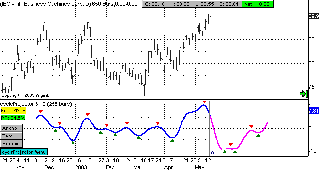
Here is a sample projection made for IBM (Daily Bars) on about 5/16/2003. High resolution was used with a 256-bar data window and we elected to to combine the 8 strongest cycles into the synthetic time series. You can see that IBM has been in a strong move up that has lasted well over a month. By eyeballing the back-plot and referring to the Fit indicator, we can see that we have a reasonably good fit over the past 120 bars of data. The cycles are indicating that a downward move is imminent.

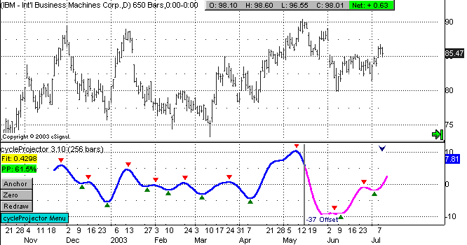
Now we move ahead in time and we can see that the projection was quite accurate in terms of direction, even up to 30+ days into the future. First of all, it correctly projected the swing down in early June as well as the subsequent rise into some minor consolidation in late June/early July. Look at the arrows on the projection.... they are all fairly close to the actual points in time where price turned around.

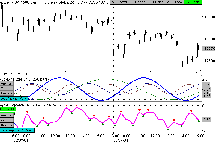
Here is a projection made on the S&P EMini (5-min bars). In this projection we are using both cycleAnalyzer and cycleProjectorXT. We anchored the projection on the 9:40am bar on 02/03/2004 and let it extend for two full days. Now, we would never use a projection this long in our trading, but it is interesting to see how well both of the projections track with the price action even two days into the future!

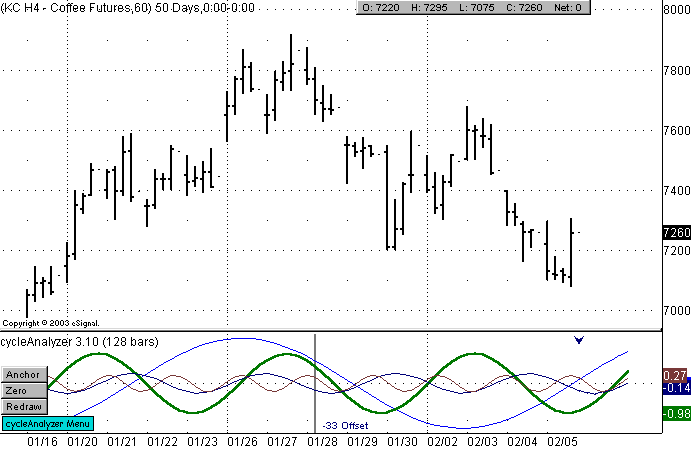
This last example is a 60-min chart of Coffee futures. Projection was made around 10:00am on 01/28/2004. See how well cycleAnalyzer projected the action over the next several days.
Good, tradable projections can be found in practically any security and on any time frame from 1-min bars to monthly bars. If the security has any kind of 'natural rhythm', the cyclePack indicators will find it. The more you work with the cycleAnalyzer and cycleProjector indicators, the better you will become at interpreting the projections and the better you will become at applying them profitably to your trading.
Copyright © 2010-2013 Divergence Software, Inc.